
This article is part of the Delay Analysis 101 series, which is also available as a LinkedIn newsletter.
In the forensic scheduling world, two pieces of literature are regularly quoted when it comes to relying on a standard method of delay analysis: the Delay and Disruption Protocol (2017) of the Society of Construction Law (SCL), and the International Recommended Practice 29R-03 on Forensic Schedule Analysis (2011) of the Association for the Advancement of Cost Engineering (AACE). This article focuses on the methods described in the SCL Delay and Disruption Protocol (the “SCL Protocol”).
In previous articles, we have seen that delay measurements can follow distinct perspectives. We have also seen that critical paths could follow distinct perspectives too. In this two-part article, we will see which method relies on which delay and critical path perspective, and what are the consequences of choosing one combination over another.
Note: Some display glitches have been reported with the display of animated images via the LinkedIn phone App. Watch via the LinkedIn web page for the best experience.
When it comes to determining causality between an event and a project delay, the SCL Protocol considers 6 delay analysis methods, namely:
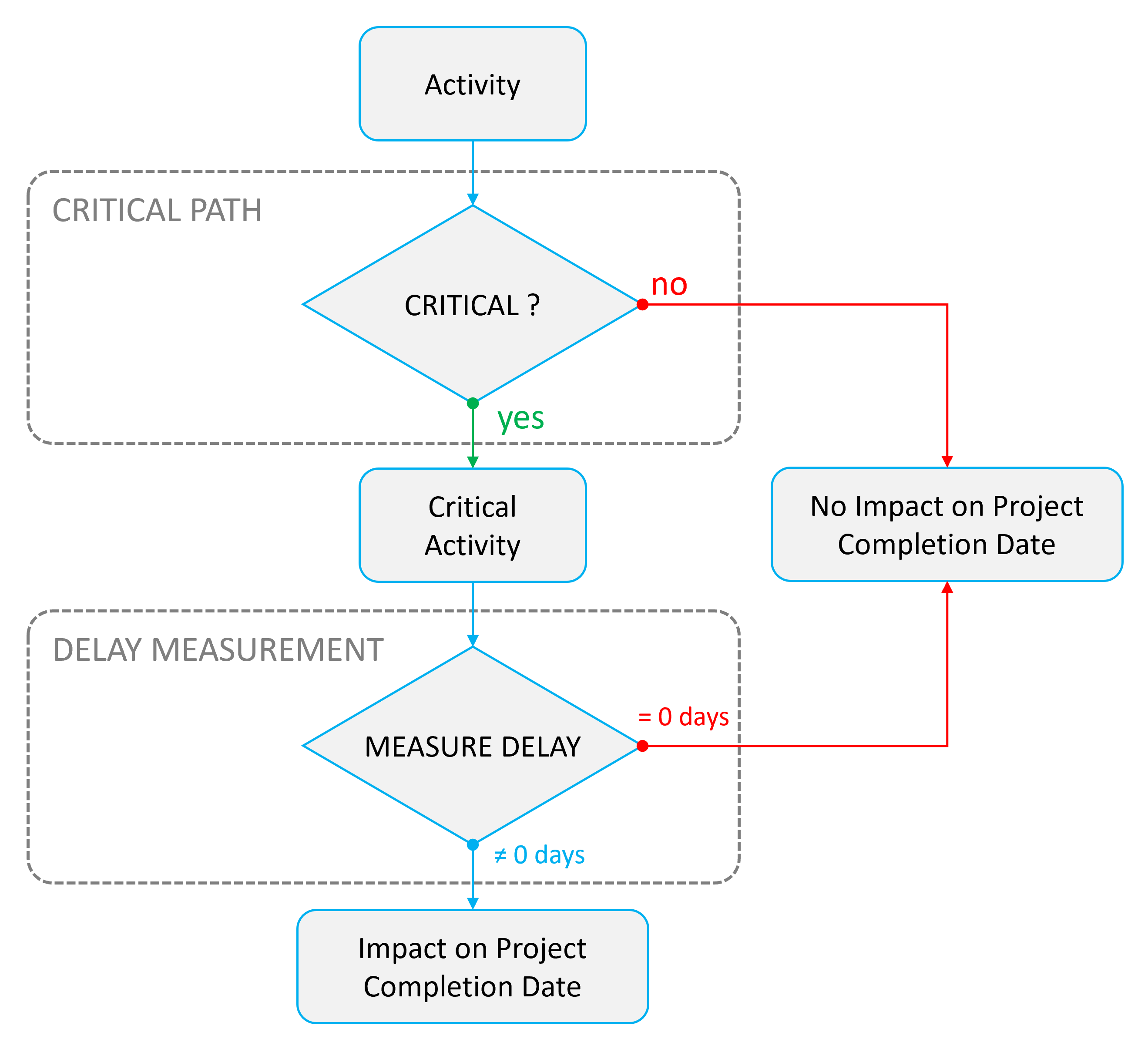
Although the implementation details and measurement methods may vary, all these methods rely on measuring delays along a critical path. For a given activity affected by a delay event, it may only impact the completion date of the project if it is critical. Yet, this condition is not sufficient because if the critical activity does not suffer delays, no impact is felt on the project completion date either. This typical flow of a delay analysis is illustrated below.
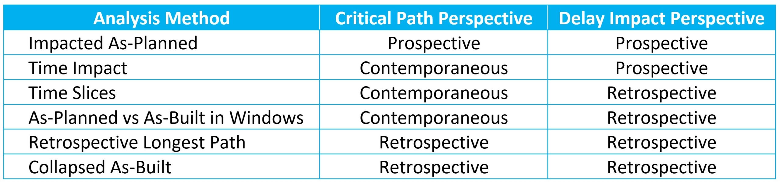
The table presented below is based on the table provided at paragraph 11.5, page 34 of the SCL Delay and Disruption Protocol (2017). This table is particularly noteworthy because it provides a concise summary of the perspectives used in each delay analysis method. It is one of my personal favourites from the SCL Protocol and it is also one of the most frequently shared extracts.
This table demonstrates how critical path and delay assessment are two separate elements of a delay analysis, and how varying combinations of perspectives may coexist.
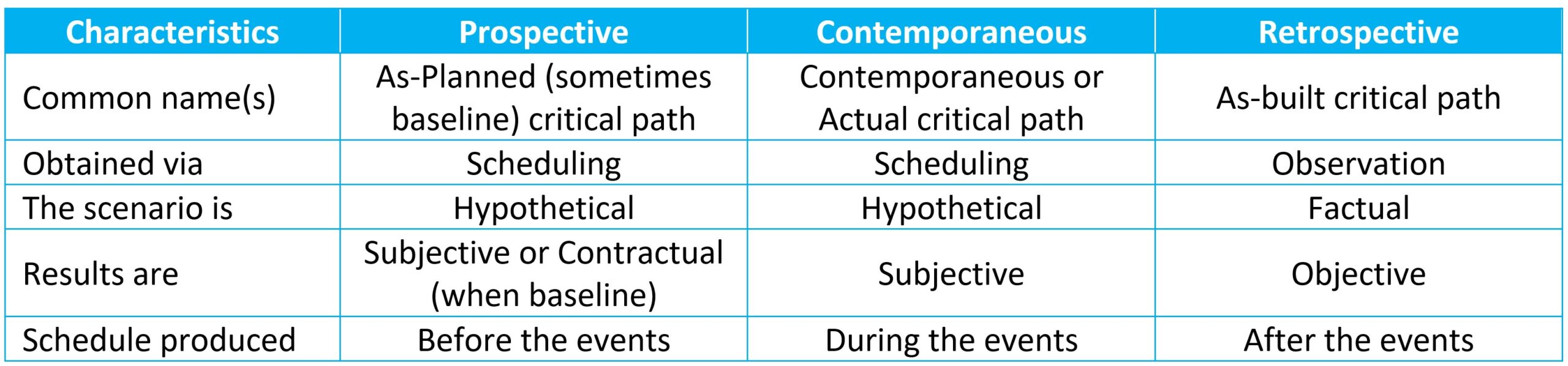
The choice of the critical path perspective defines what schedule to use in order to identify the sequence of activities which mattered for the analysis:
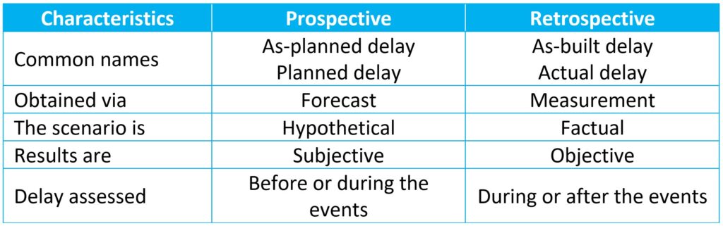
The choice of the delay measurement perspective defines which impact of the delay events matters:
The six delay analysis methods considered by the SCL Protocol rely on varying combinations of critical path and delay analysis perspectives because they address different questions.
In future articles, we will delve into the specific steps required to implement each method fully. For now, we will touch on the fundamental principles behind each approach but remain at an introductory level.
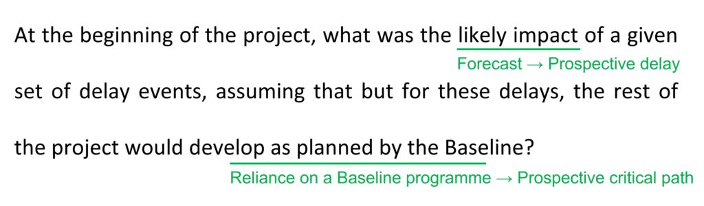
This method answers a question which could be phrased as follows:
At the beginning of the project, what was the likely impact of a given set of delay events, assuming that but for these delays, the rest of the project would develop as planned by the Baseline?
A review of this question already gives us a good feel for what perspectives are used. The method focuses on a likely impact, which means it assesses delays based on a forecast: delay is prospective, i.e. as-planned. The programme relied upon is that of the Baseline, which means the critical path is inferred from this programme and is therefore prospective, or as-planned.
The general idea is to inject delay events inside the Baseline programme and compare the project completion date of the original Baseline with the now impacted Baseline.
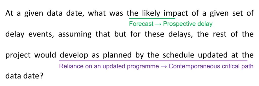
This method answers a question which could be phrased as follows:
At a given data date, what was the likely impact of a given set of delay events, assuming that but for these delays, the rest of the project would develop as planned by the schedule updated at the data date?
Just like the impacted as-planned method, the time impact method focuses on a likely impact, which means it assesses delays based on a forecast: delay is prospective, i.e. as-planned. The programme relied upon is one updated close to the data date, which means the critical path is inferred from this programme and is therefore contemporaneous.
The general idea is to inject delay events inside the contemporaneous programme and compare the project completion date of the contemporaneous programme with the now impacted contemporaneous programme.
In the second part of this article, we will address the time slices, the as-planned versus as-built in windows, the retrospective longest path, and the collapsed as-built delay analysis methods. Visit for more content like this one.

Construction delay expert Amaël Olivier is the Founding partner of Orizo Consult International. He cumulates over a decade of delay analysis know-how, including the review of major landmark projects across more than 25 countries. He excels in complex infrastructure and energy investments, having assessed projects ranging from 10 to 3,500 million USD in capital value. He testifies in English, French, and Spanish.
The concepts presented in this article are orientative and have been simplified for the purpose of addressing a wide audience. The opinions are those of the author at the time of writing, not necessarily those of Orizo Consult International. Each case includes its own particularities, which is why we do not pretend to be providing professional advice through this content.